Get Started

library(mrgsim.ds)
library(dplyr)

Overview

mrgsim.ds provides an Apache Arrow-backed simulation output object for mrgsolve, greatly reducing the memory footprint of large simulations and providing a high-performance pipeline for summarizing huge simulation outputs. The arrow-based simulation output objects in R claim ownership of their files on disk. Those files are automatically removed when the owning object goes out of scope and becomes subject to the R garbage collector. While “anonymous”, parquet-formatted files hold the data in tempdir() as you are working in R, functions are provided to move this data to more permanent locations for later use.

Load a model

Load a model using mread_ds() or other friends.

mod <- mread_ds("popex-2.mod", outvars = "IPRED, DV, ECL")

This model is almost identical to the same model loaded with mread(); there is just some extra information included in the model object to make sure it works well with the mrgsim.ds approach.

Other functions you can use to load a model include

These all mimic the corresponding functions in mrgsolve.

Simulate

To simulate, call mrgsim_ds(); all arguments get passed to mrgsim().

data <- evd_expand(amt = c(100, 300, 700), ii = 24, addl = 4, ID = 1:10)

data <- mutate(data, dose = AMT)

set.seed(98)
out <- mrgsim_ds(mod, data = data, end = 5*24, recover = "dose")

The output behaves very similarly to regular mrgsim() output.

out

## Model: popex-2_mod
## Dim  : 7,260 x 6
## Files: 1 [140.2 Kb]
## Owner: yes (gc)
##     ID TIME        ECL     IPRED        DV dose
## 1:   1  0.0 -0.1397334 0.0000000 0.0000000  100
## 2:   1  0.0 -0.1397334 0.0000000 0.0000000  100
## 3:   1  0.5 -0.1397334 0.7493918 0.7493918  100
## 4:   1  1.0 -0.1397334 1.2650920 1.2650920  100
## 5:   1  1.5 -0.1397334 1.6175329 1.6175329  100
## 6:   1  2.0 -0.1397334 1.8559447 1.8559447  100
## 7:   1  2.5 -0.1397334 2.0147377 2.0147377  100
## 8:   1  3.0 -0.1397334 2.1179631 2.1179631  100

head(out)

## # A tibble: 6 × 6
##      ID  TIME    ECL IPRED    DV  dose
##   <dbl> <dbl>  <dbl> <dbl> <dbl> <dbl>
## 1     1   0   -0.140 0     0       100
## 2     1   0   -0.140 0     0       100
## 3     1   0.5 -0.140 0.749 0.749   100
## 4     1   1   -0.140 1.27  1.27    100
## 5     1   1.5 -0.140 1.62  1.62    100
## 6     1   2   -0.140 1.86  1.86    100

tail(out)

## # A tibble: 6 × 6
##      ID  TIME      ECL IPRED    DV  dose
##   <dbl> <dbl>    <dbl> <dbl> <dbl> <dbl>
## 1    30  118. -0.00385  19.4  19.4   700
## 2    30  118  -0.00385  19.0  19.0   700
## 3    30  118. -0.00385  18.5  18.5   700
## 4    30  119  -0.00385  18.1  18.1   700
## 5    30  120. -0.00385  17.7  17.7   700
## 6    30  120  -0.00385  17.2  17.2   700

dim(out)

## [1] 7260    6

names(out)

## [1] "ID"    "TIME"  "ECL"   "IPRED" "DV"    "dose"

plot(out, nid = 10)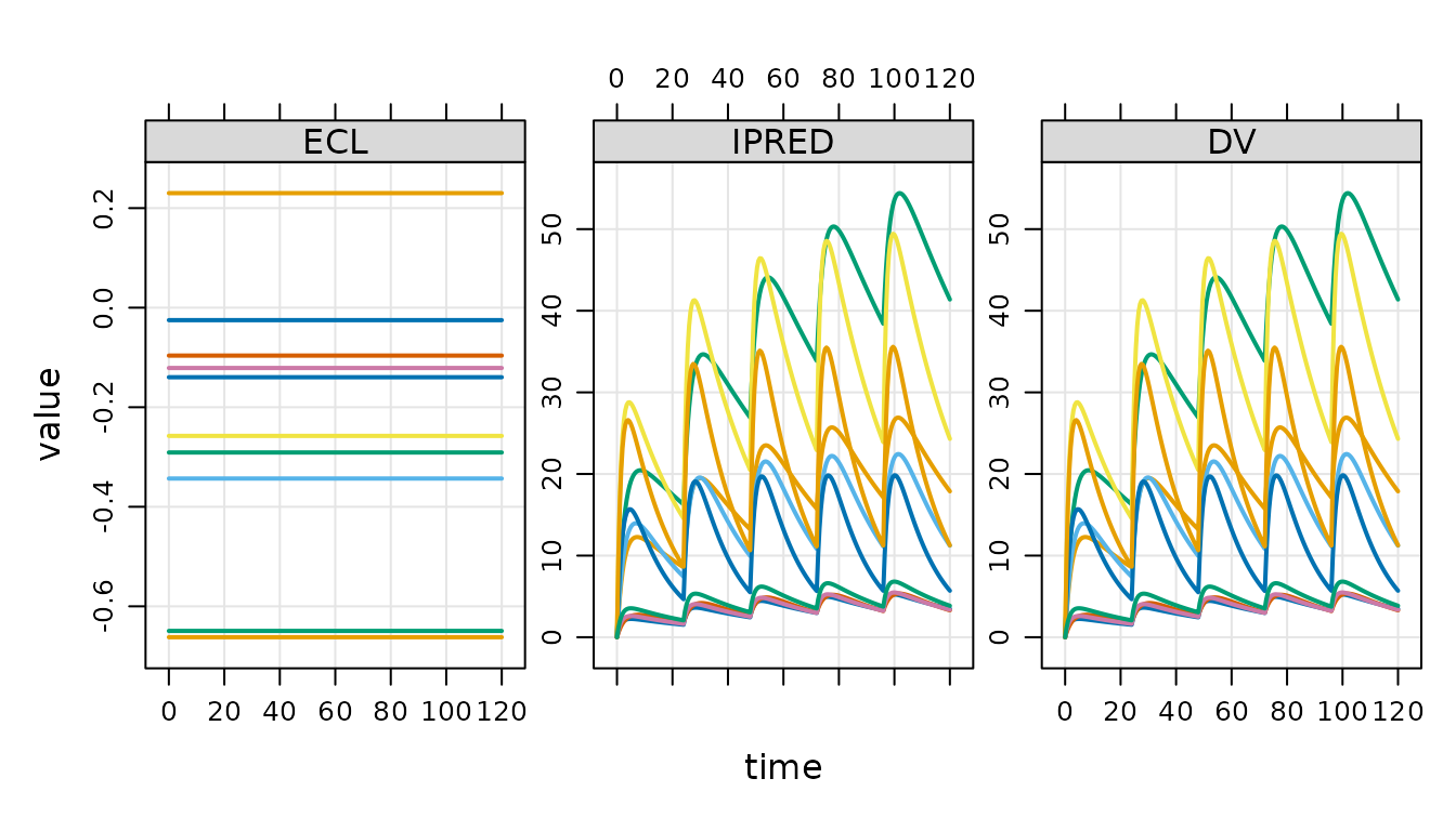

out owns the file that contains the simulated data.

ownership()

## > Objects: 1 | Files: 1 | Size: 140.2 Kb

check_ownership(out)

## [1] TRUE

This object is an environment and therefore is modified by reference. If you want to make a copy of this object, use copy_ds().

out2 <- copy_ds(out, own = TRUE)

You can specify which object will own the files on copy.

Summarizing outputs with arrow

mrgsim.ds provides access points to dplyr / arrow data wrangling pipelines.

out %>% 
  filter(TIME == 5*24) %>% 
  select(TIME, dose, IPRED) %>% 
  group_by(dose) %>% 
  summarise( 
    Min = min(IPRED), 
    Mean = mean(IPRED), 
    Max = max(IPRED), 
    .groups = "drop"
  ) %>% collect()

## # A tibble: 3 × 4
##    dose   Min  Mean   Max
##   <dbl> <dbl> <dbl> <dbl>
## 1   100  2.02  3.39  4.97
## 2   300  5.70 10.6  17.9 
## 3   700  7.29 18.6  41.4

Note that we must call collect() or as_tibble() here in order to realize the summarized results.

See the Arrow documentation for more details on these Arrow pipelines. For now, note that if you want exact quantile summaries (including median), you have to convert to a duckdb object. This is cheap and easy to do with the as_duckdb_ds() function.

out %>% 
  as_duckdb_ds() %>% 
  filter(TIME == 5*24) %>% 
  select(TIME, dose, IPRED) %>% 
  group_by(dose) %>% 
  summarise( 
    P5 = quantile(IPRED, 0.05, na.rm = TRUE), 
    Mean = mean(IPRED), 
    Median = median(IPRED),
    P95 = quantile(IPRED, 0.95, na.rm = TRUE), 
    .groups = "drop"
  ) %>% collect()

## Warning: Missing values are always removed in SQL aggregation functions.
## Use `na.rm = TRUE` to silence this warning
## This warning is displayed once every 8 hours.

## # A tibble: 3 × 5
##    dose    P5  Mean Median   P95
##   <dbl> <dbl> <dbl>  <dbl> <dbl>
## 1   100  2.03  3.39   3.42  4.97
## 2   700  7.93 18.6   16.8  35.8 
## 3   300  6.74 10.6   10.3  15.5

If you only want to get your simulated data as an R data frame, simply coerce to tibble.

as_tibble(out)

## # A tibble: 7,260 × 6
##       ID  TIME    ECL IPRED    DV  dose
##    <dbl> <dbl>  <dbl> <dbl> <dbl> <dbl>
##  1     1   0   -0.140 0     0       100
##  2     1   0   -0.140 0     0       100
##  3     1   0.5 -0.140 0.749 0.749   100
##  4     1   1   -0.140 1.27  1.27    100
##  5     1   1.5 -0.140 1.62  1.62    100
##  6     1   2   -0.140 1.86  1.86    100
##  7     1   2.5 -0.140 2.01  2.01    100
##  8     1   3   -0.140 2.12  2.12    100
##  9     1   3.5 -0.140 2.18  2.18    100
## 10     1   4   -0.140 2.22  2.22    100
## # ℹ 7,250 more rows

If you want the arrow data set object:

as_arrow_ds(out)

## FileSystemDataset with 1 Parquet file
## 6 columns
## ID: double
## TIME: double
## ECL: double
## IPRED: double
## DV: double
## dose: double
## 
## See $metadata for additional Schema metadata

If you want an arrow table object:

arrow::as_arrow_table(out)

## Table
## 7260 rows x 6 columns
## $ID <double>
## $TIME <double>
## $ECL <double>
## $IPRED <double>
## $DV <double>
## $dose <double>
## 
## See $metadata for additional Schema metadata

Working with lists of objects

mrgsim.ds provides utilities for working with lists of output objects that are typically realized when simulating replicates in parallel.

Here are 10 simulation replicates.

out <- lapply(1:10, \(x) mrgsim_ds(mod, data))

Because we used lapply(), the result is a list of simulation output objects

class(out)

## [1] "list"

We’d like to work with these simulations as a single object. To do that, use reduce_ds()

out <- reduce_ds(out)

This leaves the backing files where they are, but creates a single object that now holds a single pointer to all 10 files.

Working with simulation files

In the last simulation, we created a list of output objects and then reduced that list to a single object with the outputs held in 10 parquet files. You can see these files when they are in tempdir().

list_temp()

## 10 files [2.9 Mb]
## - mrgsims-ds-1bbd10b4be8e.parquet
## - mrgsims-ds-1bbd204e628a.parquet
##    ...
## - mrgsims-ds-1bbd5dd1b150.parquet
## - mrgsims-ds-1bbd6a9e985.parquet

Or get a list of the files as an R character vector:

files_ds(out)

##  [1] "/tmp/RtmpCw7sHd/mrgsims-ds-1bbd3cb565a2.parquet"
##  [2] "/tmp/RtmpCw7sHd/mrgsims-ds-1bbd204e628a.parquet"
##  [3] "/tmp/RtmpCw7sHd/mrgsims-ds-1bbd10b4be8e.parquet"
##  [4] "/tmp/RtmpCw7sHd/mrgsims-ds-1bbd56a55833.parquet"
##  [5] "/tmp/RtmpCw7sHd/mrgsims-ds-1bbd2bd147d7.parquet"
##  [6] "/tmp/RtmpCw7sHd/mrgsims-ds-1bbd5dd1b150.parquet"
##  [7] "/tmp/RtmpCw7sHd/mrgsims-ds-1bbd2fde8bb0.parquet"
##  [8] "/tmp/RtmpCw7sHd/mrgsims-ds-1bbd6a9e985.parquet" 
##  [9] "/tmp/RtmpCw7sHd/mrgsims-ds-1bbd29263da7.parquet"
## [10] "/tmp/RtmpCw7sHd/mrgsims-ds-1bbd32f1529f.parquet"

To save outputs to a persistent location, use save_ds().

save_ds(out, file = file.path(save_dir, "sims.rds"))

This creates an .rds file holding the (very lightweight) simulation output object and it relocates all the backing files to save_dir.

To read the simulations back into R:

bah <- read_ds(file.path(save_dir, "sims.rds"))

bah

## Model: popex-2_mod
## Dim  : 144.6K x 5
## Files: 10 [2.9 Mb]
## Owner: yes (no gc)
##     ID TIME        ECL    IPRED       DV
## 1:   1  0.0 -0.0317765 0.000000 0.000000
## 2:   1  0.0 -0.0317765 0.000000 0.000000
## 3:   1  0.5 -0.0317765 1.851493 1.851493
## 4:   1  1.0 -0.0317765 2.833834 2.833834
## 5:   1  1.5 -0.0317765 3.338411 3.338411
## 6:   1  2.0 -0.0317765 3.580684 3.580684
## 7:   1  2.5 -0.0317765 3.679257 3.679257
## 8:   1  3.0 -0.0317765 3.699414 3.699414

An alternative is to rename and move.

rename_ds(bah, "regimen-1")
move_ds(bah, save_dir)

## ℹ 10 files are now located in /tmp/RtmpCw7sHd; gc is off.

If you want all the simulated data output in a single parquet file that you name and locate.

write_parquet_ds(x = bah, sink = "new/path/file.parquet")

Garbage collection

## Discarding 10 files.

When a new simulation output object is created, that object owns the files and, by default, the files will be deleted as soon as the object goes out of scope. The files are deleted when the R garbage collector is called.

out <- mrgsim_ds(mod, data)

out

## Model: popex-2_mod
## Dim  : 14,460 x 5
## Files: 1 [295 Kb]
## Owner: yes (gc)
##     ID TIME        ECL    IPRED       DV
## 1:   1  0.0 -0.3538907 0.000000 0.000000
## 2:   1  0.0 -0.3538907 0.000000 0.000000
## 3:   1  0.5 -0.3538907 1.456466 1.456466
## 4:   1  1.0 -0.3538907 2.388291 2.388291
## 5:   1  1.5 -0.3538907 2.977009 2.977009
## 6:   1  2.0 -0.3538907 3.341447 3.341447
## 7:   1  2.5 -0.3538907 3.559382 3.559382
## 8:   1  3.0 -0.3538907 3.681724 3.681724

You can see that out owns the files and they are marked for garbage collection when appropriate.

output_files <- files_ds(out)

file.exists(output_files)

## [1] TRUE

Let’s blow away out and check the files.

rm(out)

gc()

##           used  (Mb) gc trigger (Mb) max used  (Mb)
## Ncells 2025442 108.2    4024487  215  4024487 215.0
## Vcells 3761556  28.7    8388608   64  6397226  48.9

file.exists(output_files)

## [1] FALSE

You can ask mrgsim.ds to notify you when the file gc is called. We won’t see the message output in this vignette, but you can confirm it in your R session.

out <- mrgsim_ds(mod, data)

out <- gc_ds(out, notify = TRUE)

rm(out)

gc()

##           used  (Mb) gc trigger (Mb) max used  (Mb)
## Ncells 2024835 108.2    4024487  215  4024487 215.0
## Vcells 3755531  28.7    8388608   64  6397226  48.9

[mrgsim.ds] cleaning up 1 file(s) ...

You can prevent the file gc from removing the files.

out <- mrgsim_ds(mod, data)

out <- gc_ds(out, value = FALSE)

out

## Model: popex-2_mod
## Dim  : 14,460 x 5
## Files: 1 [295 Kb]
## Owner: yes (no gc)
##     ID TIME        ECL    IPRED       DV
## 1:   1  0.0 -0.2222274 0.000000 0.000000
## 2:   1  0.0 -0.2222274 0.000000 0.000000
## 3:   1  0.5 -0.2222274 1.212429 1.212429
## 4:   1  1.0 -0.2222274 2.084579 2.084579
## 5:   1  1.5 -0.2222274 2.706065 2.706065
## 6:   1  2.0 -0.2222274 3.143001 3.143001
## 7:   1  2.5 -0.2222274 3.444165 3.444165
## 8:   1  3.0 -0.2222274 3.645541 3.645541

Now, your files will remain after the object goes out of scope. But remember that, in this example, the files are still in tempdir() and they will be blown away when R restarts. So if you really want to keep the output files safe, it’s best to use save_ds(), move_ds(), or write_parquet_ds() to relocate files out of tempdir(), while also disabling file garbage collection.